When you are a statistician and your spouse is convinced that his luck at poker is worse than normal, you tell him about observational bias, the importance of data collection before drawing conclusions, how easy it is to remember the losses and forget the wins, etc. Then, when he keeps insisting and starts collecting data, you help him figure out a way to test his suspicion.
Ideally what will happen is he’ll collect some data, realize the data is in line with the expectations of random chance and reconsider his perceptions. But, in my husband’s case, the data just keeps confirming that his observations were accurate. Every measure we devise to test the hypothesis remains stubbornly on the low side of a reasonable probability.
The graph below (figure 1) shows the expected probability of winning on the x-axis and the actual % of wins on y-axis. Points below the diagonal are sessions when his luck was worse than expected while the points above the diagonal are sessions when his luck was better than expected. The red dot and the purple X mark the average of both with 95% confidence limits for the 2013 and 2014 data sets respectively.
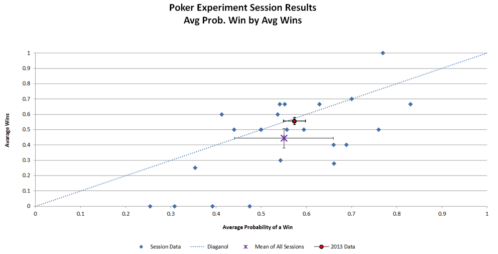
Figure 1
Thus, we are now facing the problem of not how to change his perception, which matches our data collection results. Instead, we should work on figuring out how to change his luck. So far, he’s had no luck with that. In fact, he doesn’t actually believe it’s possible. I am more optimistic. I think we may have some capability to create our own luck.
Defining Luck: First of all, we define luck as an average of a measurable probabilistic outcome that is purely due to change alone – i.e. unaffected by any knowledge or skill displayed. Next, we define bad luck as a measure of luck that is significantly different from the expected values predicted by random chance with a 1−α% level of confidence. 1−α% can be set to whatever extreme probability we wish before concluding that the results are NOT due to random chance alone.
In order to obtain a probability outcome due to luck alone (we wanted to divorce skill from our measurement in order to ascertain luck by itself), we used the results of an all-in call in Texas Holdem poker. After this call is made, the players cards are face up on the table and the probability of win can be computed exactly whilst completely unaffected by any play after this point.
Data Coding: Game outcomes were scored as wins equal 1, losses at 0, and ties at 0.5. The expected probability for each hand at the time the all-in was called was computed at http://www.cardplayer.com/poker-tools/odds-calculator/texas-holdem. In the values shown in Figure 1, the probability of a tie is included, with the probability of a tie weighted at 0.5.
Data Collection: My husband plays poker (Texas Hold’em) twice a month in a buddy’s garage. Each night of poker comprises two or sometimes three tournaments. This is the data referred to as live hands or sessions. So he wrote down the cards involved for every all-in hand he played over the course of a year. [1]
He also frequently plays on-line poker at fulltiltpoker.com. The game play data could be be saved to a computer file.
Starting back in 2012, I convinced him to collect data on every all-in hand. For over a year, he collected data on both his on-line and live games played. I painstakingly entered the probability for each hand computed when he laid down his cards. In July of 2013, he started another data collection solely on his live games. In December of 2013, I talked him into noting the live games separately from the on-line poker games.
Data Set 2013: In December of 2013 I decided I had had enough of inputting all those probabilities. At the end of the year, I would stop inputting the data from the on-line games, which was the majority of our dataset. From this point on, I would only input the data from the live hands. In January, we had data from 1,451 games. Mark had 785 wins and 44 ties.
Null Hypothesis Let p represent the average probability of a win for all 1451 games, we can compute E(p) = the average of the expected probability for each game, then compute the difference d = E(p) – p. The test statistic, d meets all required assumptions for a one-sided t-test. With n = 1451, the t distribution converges to the normal distribution.
H0: d = 0 H1: d > 0 Under H0, d ~n(0, S2/n)
Results: The theoretical mean value computed from the probabilities of the individual games, was E(p) = 0.5737. His actual mean value, computed from his wins, losses and ties, was p=0.5562. This difference of 0.0191 has a probability of 0.0672. We can reject the null hypothesis at the 90% confidence level, but not the 95% confidence level.
Data Set 2014-1 : This data is from live hands only. The hands recorded for each date constitute a session, which is our experimental unit. The mean of both the expected and actual wins was computed for each session. Since we are using the means of the session, we can assume an underlying normal distribution and use a t-test to compute the probability of the difference between the expected and actual wins.
Null Hypothesis: While the actual number of recorded all-in hands in a session varied from two to ten, the average probability and the average wins are statistics that will follow a normal distribution with an average difference of 0 under the null hypothesis. The test statistic, d, is mean of the difference between the average probability of the hands played and the average number of wins for the session. With n representing the number of sessions, not the number of games, this statistic meets all required assumptions for a one-sided paired t-test.
H0: d = 0 H1: d > 0 Under H0d ~tn(0, S2/n)
Results: The p-value is the probability of a getting a mean difference between the average probability and the average wins, given the hands dealt. Currently, as of 9-13-14, the p-value of a one-sided paired t-test on the session results is 0.0086 ~ 1 in 116. We can reject the null hypothesis that everything is normal at 99% confidence level, but not at the 99.5% confidence level.
Basically, the data we’ve collected is evidence that supports his contention that his luck is significantly worse than what is expected from random chance.
Data Set 2014-2: Another dataset, collected on the live games from July 2013 to July 2014, is the number of times he is dealt the hands {A, K} and {Q, 8} and {5, 2}[2]. These are considered to be a very good hand, an ‘average’ hand, and a very poor hand, respectively. He recorded each instance of being dealt one of these three hands. Random chance gives the expectation that each of these hands are equally probable. The results are as follows:
| Hands | Value | # Observed | # Expected | Obs. Values | Exp. Values |
| {A,K} |
21.5 |
32 |
43.333 |
688 |
931.667 |
| {Q, 8} |
10 |
39 |
43.333 |
390 |
433.333 |
| {5, 2} |
5 |
59 |
43.333 |
295 |
216.667 |
Now, even though he’s doing his best to record this data accurately, it’s possible that he’s making mistakes and forgetting to write down all the {A, K} and {Q, 8} hands. But he would have to have made A LOT of that type of mistake to bring them up to be roughly equal to the {5,2} hands. Which is hard to believe given that every time he plays {A, K}, his fellow players enjoy reminding him to write it down. I find it difficult to attribute a difference of this magnitude to data collection errors in this situation.
Comparing just the {A, K} with the {5,2} without taking into account the fact that {A, K} is a much more valuable hand that {5, 2}, the binomial probability of that sort of inequality is 0.0031. This means we can reject the null and accept the alternative – his luck is worse than expected according to random chance at the 99.5% level, but not at the 99.9% level. The difference between {A, K} and {Q, 8} was not remarkable with a binomial p-value of 0.2383, while the difference between {Q, 8} and {5, 2} was anomalous at 0.0272. In other words, he was deal {5,2} hands significantly more often than either the {A, K} with a confidence level of 99.7% or the {Q,8} with a confidence level of 97.2%.
A chi-squared test including all three hands gives a p-value of 0.0108. If values are assigned to the hands based on their worth: {A, K} = 21.5, {Q, 8} = 10, {5,2} = 5, the chi-squared test gives a p-value of 1.17734E-21. Essentially zero.
I see no conclusion but that his observations of bad luck are accurate. The next question, for me, is how do we change it? While I have no idea how to do that, I do know how to measure whether or not we are successful.
[1] We recognize that for people outside of our small band of garage poker players, a cheater in our midst seems a plausible explanation for these results. However, due to the way the garage poker game is conducted and our knowledge of the players personally, this is a hypothesis that has been rejected a priori.
[2] I tried to persuade him to write down every hand he dealt, but that slows down the game (I tried it, it does) and he did not want to impose that on his fellow poker players.